
Highlight a Whole Row Based on One Cell’s Value in Excel
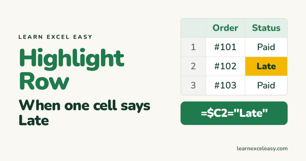
Highlight Cells Rules colour one cell. To colour the whole row when column C says Late, you need one formula rule and one dollar sign in the right place.
Steps
- Select the whole table without the heading — click A2, then Shift + click the last cell (say F200).
- Home › Conditional Formatting › New Rule.
- Choose Use a formula to determine which cells to format.
- Type:
=$C2="Late" - Click Format › Fill tab › pick a colour. OK. OK.
Every row whose column C is Late turns that colour, end to end.
Why $C2 and not C2 or $C$2
$C— always look at column C, whichever column is being painted.2without $ — move down row by row.$C$2would check only cell C2 for every row — wrong.
The row number must be the first row of your selection. Selected from row 2? Write C2. From row 5? C5.
Other conditions
| Highlight rows where… | Formula |
|---|---|
| Amount in D is over 1000 | =$D2>1000 |
| Date in E is past | =$E2<TODAY() |
| Column B is empty | =$B2="" |
| Status matches cell H1 | =$C2=$H$1 |
Check it worked
Change a Paid row to Late. It colours instantly. Change it back — colour goes.
Common mistake
Selecting the table starting at A1 but writing C2 in the formula. Everything shifts by one row. Match the formula’s row to the first selected row.

20 years with spreadsheets and enterprise systems. Writes one short, plain-English Excel lesson a day. Got an Excel question? learnexceleasycom@gmail.com
