
How to Calculate Compound Interest in Excel (formula and FV)
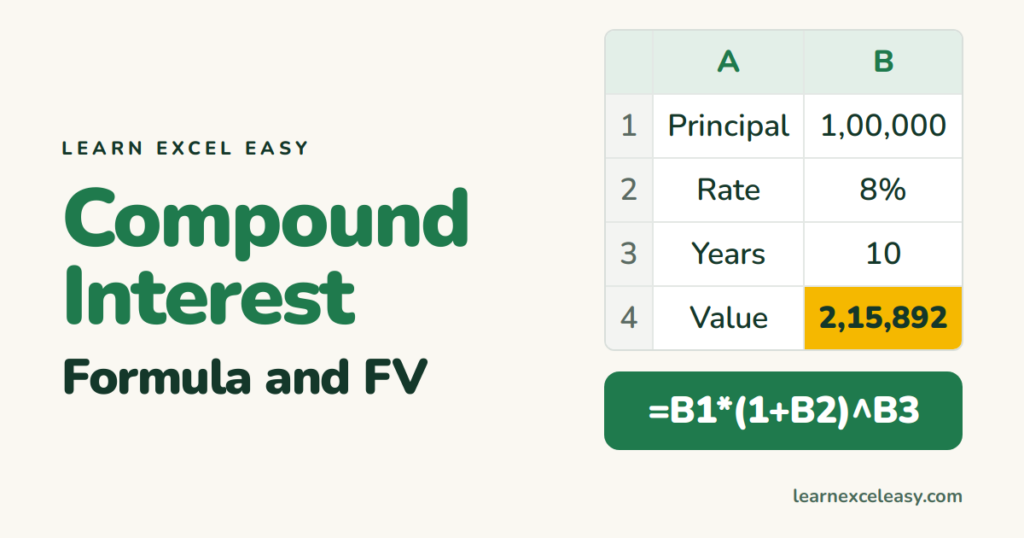
Compound interest means interest earns interest. Excel has both the textbook formula and a function that does it for you.
Set up the inputs
| A | B | |
|---|---|---|
| 1 | Principal | 100000 |
| 2 | Rate (yearly) | 8% |
| 3 | Years | 10 |
The formula (compounded yearly)
=B1 * (1 + B2) ^ B3
Result: 2,15,892. The ^ means “to the power of”.
Compounded monthly
=B1 * (1 + B2/12) ^ (B3*12)
Result: 2,21,964 — more, because interest is added 120 times instead of 10.
With FV (does the same, handles deposits)
=FV(B2/12, B3*12, 0, -B1)
Rate per period, number of periods, payment per period, present value (negative = money you put in).
With a monthly deposit of 5,000 too
=FV(B2/12, B3*12, -5000, -B1)
Interest earned only
=FV(B2/12, B3*12, 0, -B1) - B1
Year-by-year table
A6:A15 = years 1 to 10. B6: =$B$1*(1+$B$2)^A6, drag down. Select and Insert › Line chart to see the curve.
Check it worked
At 8% for 9 years money roughly doubles (rule of 72). 1,00,000 → about 2,00,000 at year 9. Yes: 1,99,900.
Common mistakes
Typing 8 instead of 8%. That is 800%. Type 8% or 0.08.
FV shows negative. You gave a positive principal. Put a minus in front of it, as above.

20 years with spreadsheets and enterprise systems. Writes one short, plain-English Excel lesson a day. Got an Excel question? learnexceleasycom@gmail.com
