Pivot Table Calculated Field in Excel: add a formula column to a pivot

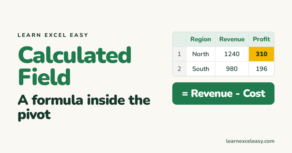
Your data has Revenue and Cost, and the pivot should show Profit. Instead of adding a column to the source, add a calculated field inside the pivot.

Steps

1. Click inside the pivot table.
2. PivotTable Analyze › Fields, Items & Sets › Calculated Field.
3. Name: Profit.
4. Formula: delete the 0, then double-click Revenue in the list, type -, double-click Cost. It reads = Revenue - Cost.
5. Click Add, then OK.

A “Sum of Profit” column appears for every row.

Margin %

Same steps, name Margin, formula = (Revenue - Cost) / Revenue. Then right-click a Margin cell › Number Format › Percentage.

Edit or delete

Open Calculated Field again, pick the name from the dropdown, change the formula › Modify, or Delete.

Check it worked

North: Revenue 1,240, Cost 930 → Profit 310. Do the subtraction by hand for one row.

The case where it is wrong

A calculated field works on sums. “Price per unit” as = Price / Units gives Sum of Price ÷ Sum of Units — not the average of each row’s price. For averages, add the column to the source data and use Average in the pivot instead.

Calculated field vs source column

Calculated field: quick, lives in the pivot, sums-only. Source column: works for anything, refreshes with the pivot, and is what Power Pivot people do. If in doubt, add the column to the data.