Sort a Pivot Table by Value in Excel (largest first)

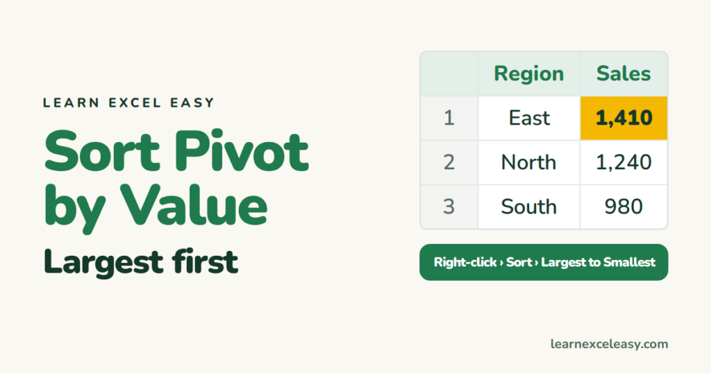
New pivots sort by label (A–Z). Two clicks sort by the numbers.

Steps

1. Right-click any number in the value column you want to sort by.
2. Sort › Sort Largest to Smallest.

Rows re-order by that value. The sort survives Refresh.

Several value columns

Right-click inside the specific column (say, Profit) and sort. The rows follow that column.

Sort with Columns in the pivot (a grid)

Right-click a value inside one column (say, North’s numbers) › Sort › More Sort Options › Largest to Smallest › More Options › untick Sort automatically if needed › choose the column. Or sort by the Grand Total column, which is the usual want.

Sort a sub-level

Region › Product in Rows: right-click a product’s value › Sort. Products sort within each region; regions stay as they were unless you sort at their level too.

Top 5 only

Click the arrow on the Row Labels heading › Value Filters › Top 10 › change 10 to 5.

Check it worked

The first row has the biggest number; each next row is smaller. Grand Total stays at the bottom.

Common mistake

Using Data › Sort A→Z on the sheet. It works once, then a refresh undoes it. Always sort from inside the pivot.