Dependent Drop-Down List in Excel (second list changes with the first)

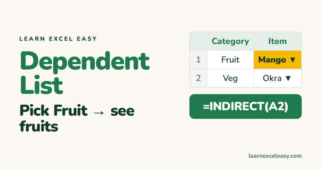
First drop-down: Fruit or Veg. Second drop-down: only fruits when Fruit is picked. Here’s how.

Method 1: named ranges + INDIRECT (every version)

Step 1 — lists. On a sheet called Lists, put each category’s items in its own column with the category as the header: Fruit in A1 with items below, Veg in B1 with items below.

Step 2 — names. Select A1:B10 › Formulas › Create from Selection › tick Top row › OK. You now have ranges named Fruit and Veg.

Step 3 — first drop-down. Select the category cells (A2:A100 on your sheet) › Data › Data Validation › List › Source: =Lists!$A$1:$B$1.

Step 4 — second drop-down. Select B2:B100 › Data Validation › List › Source:

=INDIRECT(A2)

A2 says “Fruit”, INDIRECT turns that into the range named Fruit. See INDIRECT.

Rules for names

Names can’t contain spaces. “Dry Fruit” becomes the name Dry_Fruit, so use =INDIRECT(SUBSTITUTE(A2," ","_")).

Method 2: FILTER (Excel 365)

Keep all pairs in one two-column table (Category | Item). In a spare cell, e.g. H2:

=FILTER(Lists!B2:B200,Lists!A2:A200=A2)

Point the second drop-down at =$H$2# (the # means the whole spilled list). Works for one input row; for many rows, stick with Method 1.

Clear the second choice when the first changes

Excel doesn’t do it automatically. Add conditional formatting that turns B red when =AND(B2<>"",COUNTIF(INDIRECT(A2),B2)=0).

Single drop-down basics: drop-down list