
INDEX MATCH in Excel: the lookup that works in any version
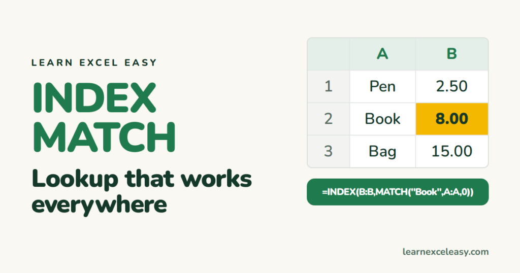
INDEX MATCH is two small formulas working together. MATCH finds which row your value is on. INDEX returns the cell from that row in another column.
Step 1: MATCH finds the row
=MATCH("Book", A1:A3, 0)
| A | B | |
|---|---|---|
| 1 | Pen | 2.50 |
| 2 | Book | 8.00 |
| 3 | Bag | 15.00 |
Result: 2. “Book” is the second item. The 0 means exact match — always use it.
Step 2: INDEX returns the value from that row
=INDEX(B1:B3, 2)
Result: 8.00. Row 2 of column B.
Put them together
=INDEX(B1:B3, MATCH("Book", A1:A3, 0))
Read it as: from column B, give me the row where column A says “Book”.
Why people use it instead of VLOOKUP
- The return column can be anywhere — left or right of the lookup column.
- Inserting or deleting columns does not break it.
- It works in every Excel version, including old ones without XLOOKUP.
Common mistake
Leaving out the 0 in MATCH. Without it Excel assumes the list is sorted and returns the wrong row without warning.
If you have Excel 2021 or 365, XLOOKUP does the same job in one formula.

20 years with spreadsheets and enterprise systems. Writes one short, plain-English Excel lesson a day. Got an Excel question? learnexceleasycom@gmail.com
