How to Reverse the Order of a List in Excel

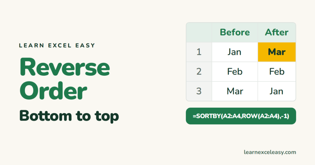
Sort Z→A reverses alphabetical order, not the order the rows are in. To flip a list upside down:

1. Helper column + sort (any Excel)

1. Next to the data, number the rows 1, 2, 3… (type 1 and 2, select both, double-click the fill handle).
2. Select everything including the numbers.
3. Data › Sort › by the helper column, Largest to Smallest.
4. Delete the helper column.

2. One formula (Microsoft 365)

=SORTBY(A2:C20,ROW(A2:A20),-1)

Stays linked to the original. For one column you can also use =CHOOSEROWS(A2:A20,SEQUENCE(ROWS(A2:A20),1,ROWS(A2:A20),-1)).

3. Older Excel formula

=INDEX($A$2:$A$20,ROWS($A$2:$A$20)-ROWS(B$2:B2)+1)

Fill down. See INDEX.

Reverse a row

=SORTBY(A1:H1,COLUMN(A1:H1),-1)

Or Data › Sort › Options › Sort left to right with a helper row.

Reverse text in a cell

=TEXTJOIN("",TRUE,MID(A2,SEQUENCE(LEN(A2),,LEN(A2),-1),1))

“Excel” → “lecxE”.

More sorting: sort in Excel · SORT