
Excel Number Format: currency, thousands separator, decimals, negative in red
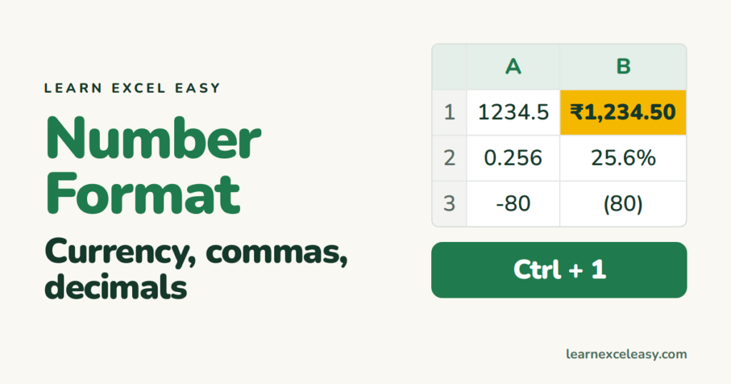
Number formats change how a value looks — not the value. 1234.5 can show as ₹1,234.50, 1,235, or 123450% and still be 1234.5 in the formula bar.
The five-second ones
| Shortcut | Format |
|---|---|
| Ctrl + Shift + 1 | Number with commas and 2 decimals |
| Ctrl + Shift + 4 | Currency |
| Ctrl + Shift + 5 | Percent |
| Ctrl + Shift + 3 | Date |
| Ctrl + Shift + ~ | Back to General |
Steps: currency with two decimals
- Select the cells.
- Press Ctrl + 1. Number tab.
- Category: Currency. Decimal places: 2. Symbol: ₹ (or $, €). OK.
More or fewer decimals
Home tab, the two buttons with .00 and arrows. Each click adds or removes one decimal place.
Thousands separator only
Ctrl + 1 › Number › tick Use 1000 separator.
Custom: negatives in red with brackets
Ctrl + 1 › Custom › type:
#,##0.00;[Red](#,##0.00)
Before the semicolon is positive, after is negative.
Indian lakhs and crores
[>=10000000]##\,##\,##\,##0;[>=100000]##\,##\,##0;##,##0
Check it worked
Click the cell. The formula bar still shows the raw number — only the cell display changed.
Common mistake
Numbers stored as text ignore all formats. Left-aligned with a green triangle? Click the icon › Convert to Number.

20 years with spreadsheets and enterprise systems. Writes one short, plain-English Excel lesson a day. Got an Excel question? learnexceleasycom@gmail.com
