
How to Use VLOOKUP in Excel: a beginner’s walkthrough
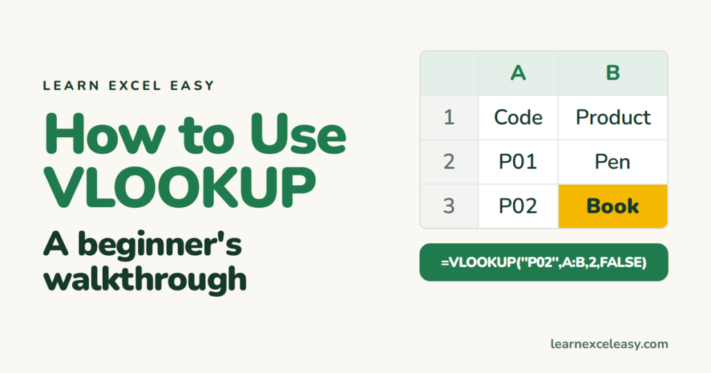
This is VLOOKUP from zero, in a blank sheet, one piece at a time. Do it as you read.
Step 1: build the lookup table
On Sheet1, type:
| A | B | |
|---|---|---|
| 1 | Code | Product |
| 2 | P01 | Pen |
| 3 | P02 | Book |
| 4 | P03 | Bag |
The thing you will search for (the code) must be in the first column.
Step 2: the cell to fill
In D1 type Code, D2 type P02. In E1 type Product. E2 is where the formula goes.
Step 3: write the formula piece by piece
Click E2 and type, in this order:
=VLOOKUP(D2,— what to findA:B,— where to look (both columns)2,— return the 2nd column of that rangeFALSE)— exact match only
=VLOOKUP(D2, A:B, 2, FALSE)
Press Enter. E2 shows Book.
Step 4: copy it down
Type more codes in D3, D4. Drag E2’s fill handle down. Each row looks up its own code.
Step 5: fix #N/A
Type P09 in D5. E5 shows #N/A — there is no P09. That is correct. To show something friendlier:
=IFERROR(VLOOKUP(D2, A:B, 2, FALSE), "Not found")
Check it worked
Change B3 from Book to Notebook. E2 changes too — the lookup is live.
Next
Newer Excel has an easier version: XLOOKUP. The full VLOOKUP reference: VLOOKUP in Excel.

20 years with spreadsheets and enterprise systems. Writes one short, plain-English Excel lesson a day. Got an Excel question? learnexceleasycom@gmail.com
