Pivot Table Count Unique Values in Excel (Distinct Count)

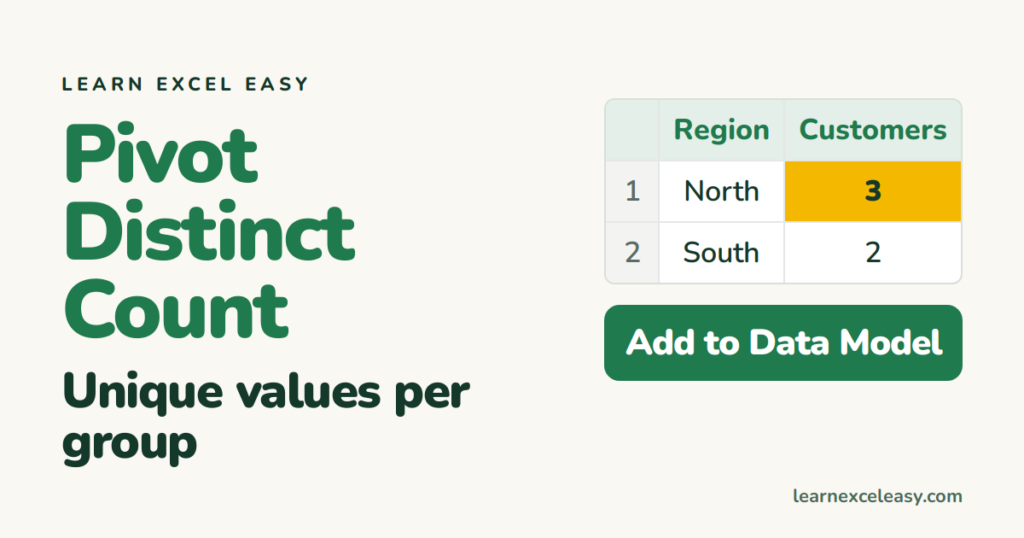
“How many different customers per region?” A normal pivot Count counts rows, so a customer with 5 orders counts 5 times. Distinct Count fixes that.

Steps (Excel 2013 and newer, Windows)

1. Click in your data. Insert › PivotTable.
2. Tick Add this data to the Data Model at the bottom. OK.
3. Drag Region to Rows, Customer to Values.
4. Click the Customer field in Values › Value Field Settings › scroll to the bottom › Distinct Count. OK.

Each region shows how many different customers it has.

Forgot the tick box?

Distinct Count is missing from the list. Delete the pivot and make it again with the box ticked — there is no way to add it afterwards.

Mac or older Excel: helper column

1. Sort the data by Region, then Customer.
2. Add a column First: =IF(COUNTIFS($A$2:A2,A2,$B$2:B2,B2)=1,1,0) — 1 the first time a region+customer pair appears, 0 after.
3. Pivot: Region to Rows, First to Values as Sum.

Check it worked

Filter the source to one region and count the unique customers by eye (or =COUNTA(UNIQUE(...))). It must match.

Common mistake

Blank customer cells count as one “unique” value. Fill or filter them out first.

Pivot basics: make a pivot table.