How to Make a Pivot Table in Excel: summarise 1,000 rows in 30 seconds

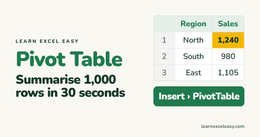
A pivot table takes a long list and gives you the totals — sales per region, orders per month — without a single formula.

What you will make

Total sales by region from a list of individual orders.

Before you start

Your list needs one heading per column, no blank rows, no merged cells. Region, Date, Product, Sales — one order per row.

Steps

1. Click any cell in the list.
2. Insert › PivotTable. Excel guesses the range. Choose New Worksheet. OK.
3. A field list appears on the right. Drag Region into the Rows box.
4. Drag Sales into the Values box.

Done. One row per region with its total.

Try these next

• Drag Product into Columns — regions down, products across, totals in the grid.
• Drag Date into Rows — Excel groups by month automatically. Right-click a date › Group to change to quarters or years.
• Click the Sales field in Values › Value Field Settings › choose Count or Average instead of Sum.
• Drag Region into Filters to get a dropdown above the table.

When the data changes

The pivot does not update by itself. Right-click it › Refresh. If you added rows below the list, first make the list an Excel Table so new rows are included.

Check it worked

Pick one region and filter the original list to it. Sum the Sales column (status bar). It must equal the pivot’s number.

Common mistakes

“Count of Sales” instead of “Sum”. One cell in the column is text or blank. Fix the data, refresh.

Blank heading. Excel refuses to build the pivot. Name every column.