
Round to the Nearest 1000 in Excel (and 100, 10, 0.5)
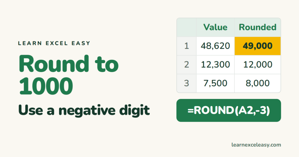
ROUND’s second number is how many decimal places to keep. Use a negative number to round to the left of the decimal point.
The formula
=ROUND(A2,-3)
| Digits | Rounds to | 48,620 becomes |
|---|---|---|
| -1 | nearest 10 | 48,620 |
| -2 | nearest 100 | 48,600 |
| -3 | nearest 1,000 | 49,000 |
| -6 | nearest million | 0 |
Always up or always down
- Up to the next 1,000:
=ROUNDUP(A2,-3)→ 48,620 becomes 49,000; 48,001 also becomes 49,000. - Down:
=ROUNDDOWN(A2,-3)→ 48,000.
More on the up direction: ROUNDUP.
Nearest 5, 50 or 0.5
- Nearest 5:
=MROUND(A2,5) - Nearest 500:
=MROUND(A2,500) - Nearest half:
=MROUND(A2,0.5) - Always up to a multiple:
=CEILING.MATH(A2,500); down:=FLOOR.MATH(A2,500)
Show thousands without changing the number
Want 48,620 to display as 49K but keep the real value for totals? Select the cells › Ctrl+1 › Custom › type #,##0,"K". One comma after the zeros divides the display by 1,000. See custom number formats.
Which one to use
Use ROUND when the rounded number feeds other calculations (prices, reports). Use the number format when only the look matters, so totals still add up exactly.

20 years with spreadsheets and enterprise systems. Writes one short, plain-English Excel lesson a day. Got an Excel question? learnexceleasycom@gmail.com
