Excel LARGE Function: top 3, top 5, 2nd highest

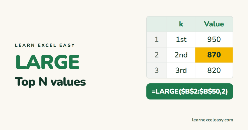
LARGE returns the k-th biggest number in a list. k=1 is the maximum, k=2 the second highest, and so on.

The formula

=LARGE(array, k)

Top 5 list

Scores in B2:B50. Type 1 to 5 in D2:D6. In E2:

=LARGE($B$2:$B$50,D2)

Copy down to E6. Lock the range with $ (why).

Second highest

=LARGE(B2:B50,2)

If the top value appears twice, LARGE(…,2) returns it again. For the second different value: =MAXIFS(B2:B50,B2:B50,"<"&MAX(B2:B50)).

Sum of the top 3

=SUM(LARGE(B2:B50,{1,2,3}))

The names that go with them

Names in A, scores in B. Next to each top value:

=INDEX($A$2:$A$50,MATCH(E2,$B$2:$B$50,0))

Ties return the first name twice. In Excel 365 the whole top-5 table is one formula:

=TAKE(SORT(A2:B50,2,-1),5)

SMALL: the lowest values

=SMALL(B2:B50,1) is the minimum, ,2) the second lowest — fastest lap times, cheapest quotes.

#NUM! error

k is bigger than the number of values, or the range has no numbers (maybe they are stored as text).