
Conditional Formatting in Excel: colour cells automatically
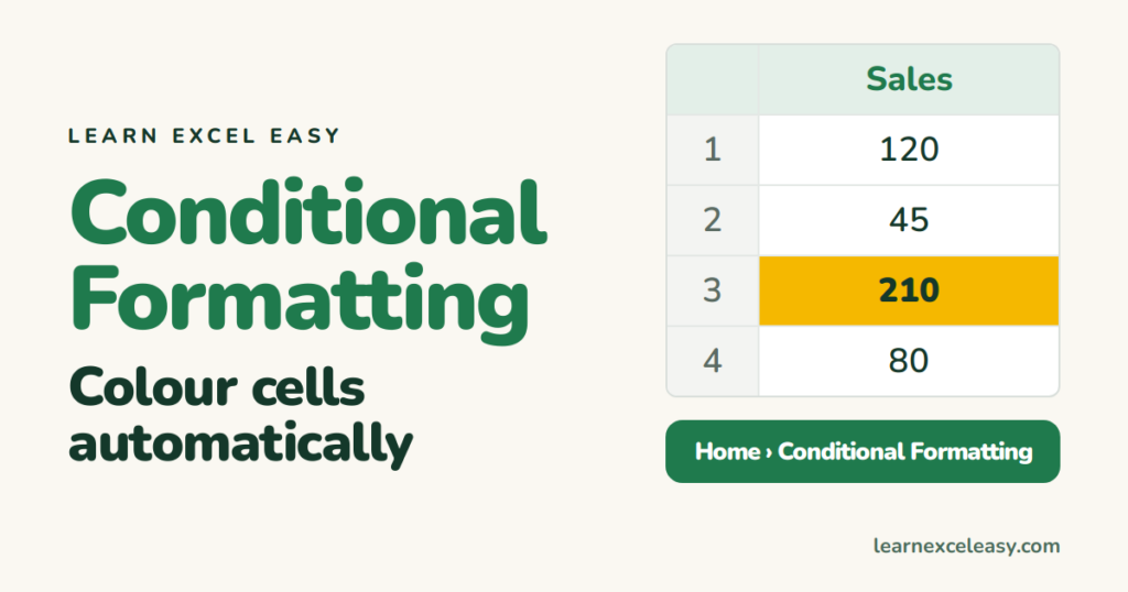
Conditional formatting colours cells by rule. Sales over 100 turn green, overdue dates turn red — automatically, as the numbers change.
Highlight values over a number
- Select the cells.
- Home › Conditional Formatting › Highlight Cells Rules › Greater Than.
- Type the number, pick a colour, OK.
Same menu: Less Than, Between, Equal To, Text that Contains, A Date Occurring, Duplicate Values.
Top 10 and above average
Conditional Formatting › Top/Bottom Rules. Top 10 Items, Top 10 %, Above Average — no formula needed.
Data bars and colour scales
Data Bars draws a bar inside each cell sized to its value. Color Scales shades low to high. Good for spotting outliers at a glance.
Colour the whole row with a formula
Select the whole table (say A2:D50). Conditional Formatting › New Rule › Use a formula. Enter:
=$D2="Late"
Pick a fill colour. Every row whose column D says Late turns that colour. The $ before D keeps the check on column D as Excel moves across the row; the missing $ before 2 lets it move down.
See or remove your rules
Conditional Formatting › Manage Rules lists everything on the sheet. Clear Rules removes them from the selection or the whole sheet.
Common mistake
The rule applies to a different range than you think. In Manage Rules, check the Applies to box and fix it there.

20 years with spreadsheets and enterprise systems. Writes one short, plain-English Excel lesson a day. Got an Excel question? learnexceleasycom@gmail.com
