Excel Alternate Row Color: stripe every other row

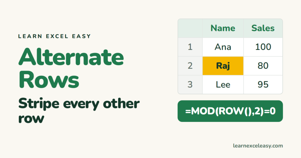
Striped rows make wide tables easier to read across. Two ways — the Table way takes five seconds.

Way 1: make it a Table

1. Click any cell in your data.
2. Press Ctrl + T. Tick “My table has headers”. OK.

Rows are striped automatically and stay striped when you sort, filter or add rows. Change the colours under Table Design › Table Styles.

Don’t want the filter arrows? Table Design › untick Filter Button.

Way 2: conditional formatting (no Table)

1. Select the range to stripe (A2:D100).
2. Home › Conditional Formatting › New Rule › Use a formula.
3. Type =MOD(ROW(),2)=0.
4. Click Format › Fill tab › pick a light colour. OK, OK.

Every even row is coloured. Use =MOD(ROW(),2)=1 for odd rows instead.

Check it worked

Insert a row in the middle. With either method the stripes re-flow — no two coloured rows touch.

Stripe columns instead

Same rule with COLUMN: =MOD(COLUMN(),2)=0. In a Table: Table Design › tick Banded Columns.

Common mistake

Painting rows by hand with the fill bucket. The moment you sort, the stripes scramble. Use one of the two methods above.