
Excel PMT Function: monthly loan or EMI payment
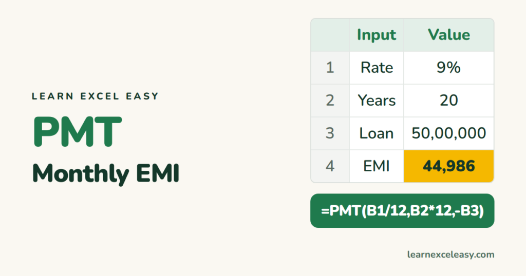
PMT gives the fixed payment per period for a loan with a constant interest rate — your EMI.
The formula
=PMT(rate, nper, pv, [fv], [type])
- rate — interest per period. Monthly payments: annual rate ÷ 12.
- nper — number of payments. 20 years monthly = 240.
- pv — the loan amount.
Example: home loan EMI
₹50,00,000 at 9% a year for 20 years. B1 = 9%, B2 = 20, B3 = 5000000:
=PMT(B1/12,B2*12,-B3)
Result: about ₹44,986 a month.
Why the minus sign
Excel follows cash flow: money you receive (the loan) is positive, money you pay is negative. Without the minus in front of B3 the EMI shows as -44,986. Either put the minus on the loan or on the whole formula.
The two classic mistakes
- Using 9% instead of 9%/12 — the payment comes out 12 times too high.
- Using 20 instead of 240 periods.
Total interest paid
=PMT(B1/12,B2*12,-B3)*B2*12-B3
About ₹57,96,600 on top of the ₹50 lakh borrowed.
Related functions
| Question | Function |
|---|---|
| Interest part of payment 1 | =IPMT(B1/12,1,B2*12,-B3) |
| Principal part of payment 1 | =PPMT(B1/12,1,B2*12,-B3) |
| How many months to repay? | =NPER(rate,payment,-loan) |
| How much can I borrow for ₹40,000/month? | =PV(B1/12,240,-40000) |
Savings growth instead of a loan: compound interest. Finding the rate that gives a target EMI: Goal Seek.

20 years with spreadsheets and enterprise systems. Writes one short, plain-English Excel lesson a day. Got an Excel question? learnexceleasycom@gmail.com
