Get the Quarter from a Date in Excel (Q1–Q4, and fiscal quarters)

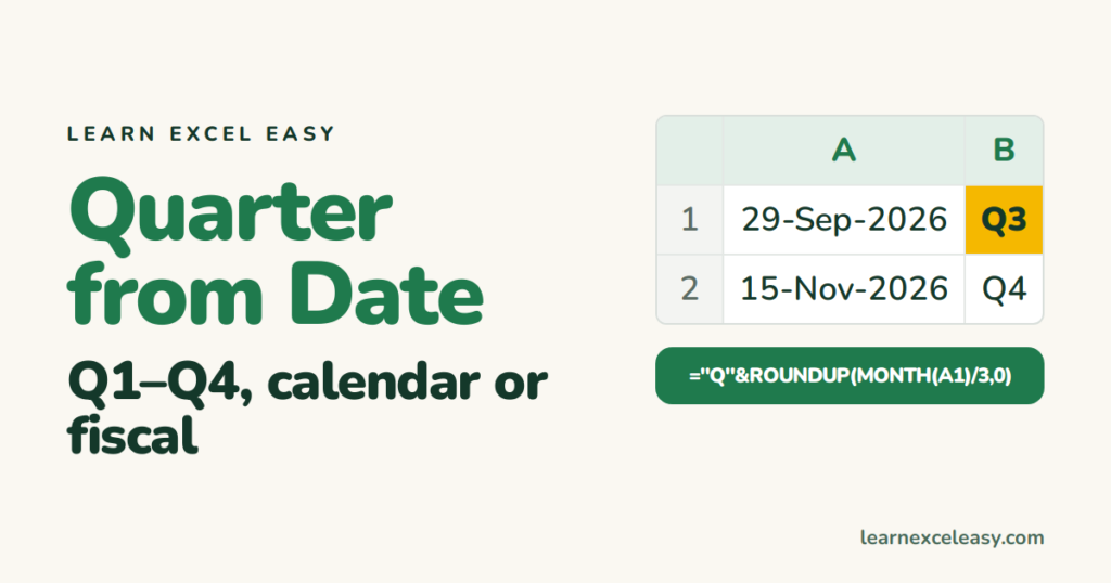
Excel has no QUARTER function, but the maths is one line.

Calendar quarter (Jan–Mar = Q1)

=ROUNDUP(MONTH(A1)/3, 0)

September is month 9; 9/3 = 3 → 3. October is 10; 10/3 = 3.33, rounded up → 4.

As text with the year

="Q" & ROUNDUP(MONTH(A1)/3,0) & " " & YEAR(A1)

→ Q3 2026. For sorting, put the year first: =YEAR(A1)&"-Q"&ROUNDUP(MONTH(A1)/3,0).

Fiscal year starting in April (India, UK)

April–June must be Q1. Shift the month by 3:

=ROUNDUP(MOD(MONTH(A1)-4, 12)/3 + 0.01, 0)

Or the readable version: =CHOOSE(MONTH(A1), 4,4,4, 1,1,1, 2,2,2, 3,3,3) — lists the quarter for each month Jan to Dec.

Fiscal year label (FY 2026-27)

="FY " & IF(MONTH(A1)>=4, YEAR(A1), YEAR(A1)-1) & "-" & TEXT(IF(MONTH(A1)>=4, YEAR(A1)+1, YEAR(A1)), "00")

Steps: total per quarter

1. Dates in A, amounts in B, quarter label in C (formula above).
2. E1: Q3 2026. F1: =SUMIF(C:C, E1, B:B).

Or a pivot: Date to Rows › right-click › Group › Quarters and Years.

Check it worked

31 March → Q1 (calendar) / Q4 (fiscal from April). 1 April → Q2 / Q1.