
Excel Pivot Table: the complete guide (build, group, filter, refresh)
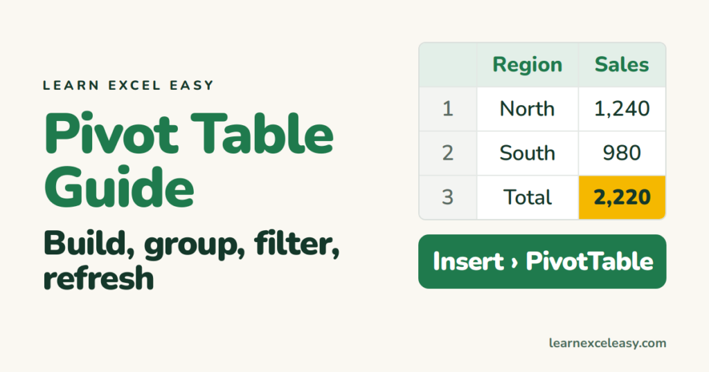
A pivot table summarises a long list — totals, counts, averages by any category — without formulas. This is the whole subject on one page; each section links to its lesson.
1. Build one (30 seconds)
Click in the data › Insert › PivotTable › OK. Drag a category to Rows, a number to Values. Step by step.
2. The four boxes
| Box | Puts the field… |
|---|---|
| Rows | down the left (one row per value) |
| Columns | across the top |
| Values | in the grid, summed (or counted) |
| Filters | in a dropdown above the table |
3. Sum, count, average, %
Click the field in Values › Value Field Settings. Show Values As › % of Grand Total for shares. If it says Count when you wanted Sum, the column has text or blanks — fix and refresh.
4. Group dates
Drag Date to Rows; Excel groups by month. Right-click a date › Group › choose Quarters, Years. Ungroup to get raw dates back.
5. Filter and slicers
Filters box = a dropdown. PivotTable Analyze › Insert Slicer = clickable buttons, nicer for dashboards. Timeline = a slicer for dates.
6. Sort
Right-click a value › Sort › Largest to Smallest. Details.
7. Calculated fields
Profit = Revenue − Cost inside the pivot. How, and when it gives wrong averages.
8. Distinct count
Tick “Add to Data Model” when creating. How.
9. Refresh
Pivots do not update by themselves. Right-click › Refresh, or Data › Refresh All. New rows below the source are missed unless the source is an Excel Table.
10. Several sheets
Stack them with Power Query first. How.
11. Pull one number out
12. Make it look normal
PivotTable Analyze › Options › Display › tick Classic layout for a flat grid. Design › Report Layout › Tabular Form; Repeat All Item Labels.
The mistakes
- Blank heading in the source → cannot create.
- Merged cells in the source → wrong groups.
- Typing into the pivot → not allowed; change the source.
- Forgetting Refresh → stale numbers.

20 years with spreadsheets and enterprise systems. Writes one short, plain-English Excel lesson a day. Got an Excel question? learnexceleasycom@gmail.com
