How to Highlight Duplicates in Excel (in one column or whole rows)

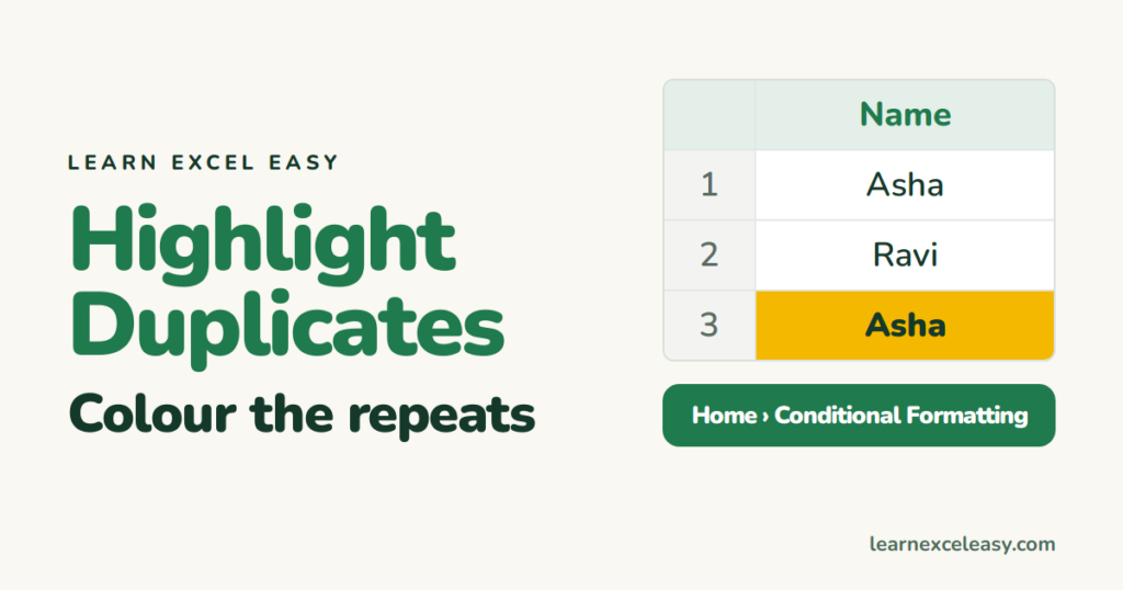
The fastest way to see duplicates is to colour them.

The 3-click way

1. Select the column (or range).
2. Home › Conditional Formatting › Highlight Cells Rules › Duplicate Values.
3. Pick a colour › OK.

Every value that appears more than once is coloured — including the first copy. The colour updates as you type.

Change “Duplicate” to Unique in the same box to colour the values that appear only once.

Only the 2nd and later copies

Select A2:A500 › Conditional Formatting › New Rule › Use a formula:

=COUNTIF($A$2:A2,A2)>1

The first occurrence stays plain; only repeats are coloured.

Whole row when a value repeats

Select the whole table (A2:F500) › New Rule › Use a formula:

=COUNTIF($A$2:$A$500,$A2)>1

The $ before A keeps the test on column A for every cell in the row. More row tricks: highlight a row based on a cell.

Duplicates across two columns

Name and date must both repeat:

=COUNTIFS($A$2:$A$500,$A2,$B$2:$B$500,$B2)>1

Remove the colour

Select the range › Conditional Formatting › Clear Rules › Clear Rules from Selected Cells.

Filter by the colour

Turn on a filter › column arrow › Filter by Color — now you see only duplicates. See filter by colour.

Next step: remove duplicates · without colour: find duplicates with COUNTIF