Filter by Color in Excel (cell colour or font colour)

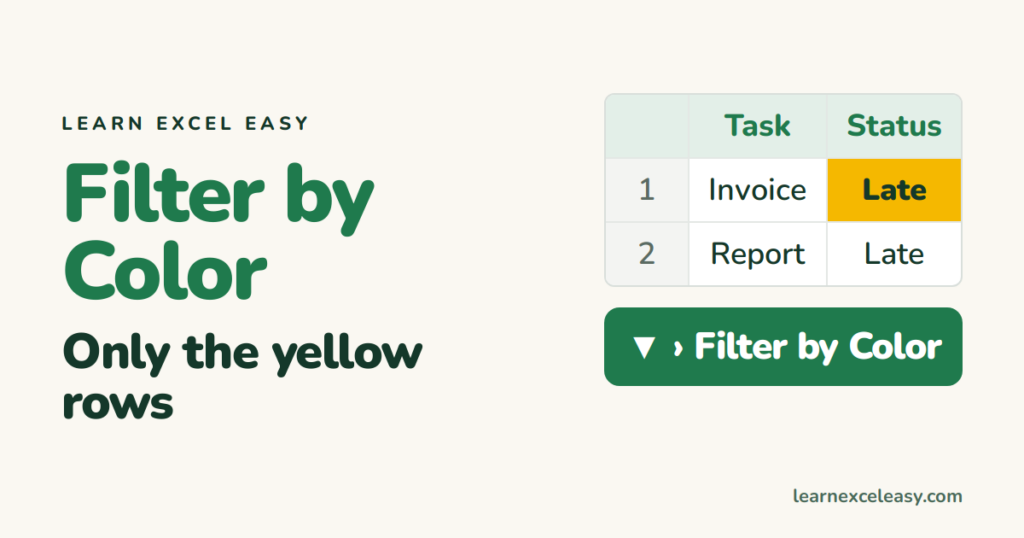
If you’ve highlighted rows by colour — by hand or with conditional formatting — you can filter to see only those.

Steps

1. Click inside the data › Ctrl+Shift+L to turn on filters.
2. Click the arrow on the coloured column.
3. Filter by Color › pick the cell colour (or font colour).

Only rows with that colour stay visible. The list shows only colours that are actually used in the column.

Font colour vs cell colour

The menu has two sections: Filter by Cell Color and Filter by Font Color. Red text is a font colour; a yellow background is a cell colour.

Cells with no colour

At the bottom of the colour list: No Fill — shows the uncoloured rows.

Only one colour at a time

You can’t pick two colours in the same filter. To see yellow and green, sort by colour instead: sort by colour puts them together at the top.

Count the coloured rows

After filtering, the status bar shows “X of Y records found”. Or in a cell: =SUBTOTAL(103,A2:A500) counts only the visible rows. See sum visible cells.

Better long term: filter by the reason, not the colour

A colour usually means something (“Late”). Put that word in a Status column and filter on the word — it survives copying to other files and works with formulas. Let conditional formatting add the colour automatically.

Clear it

Column arrow › Clear Filter From…, or Ctrl+Shift+L to turn filters off. More: filters.