Custom Number Format in Excel: K, M, text labels, colours

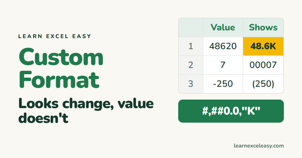
A custom number format changes how a number displays. The value underneath stays the same, so totals and formulas still work.

Where

Select the cells › Ctrl+1 › Number tab › Custom › type the code in the Type box.

Ready-to-copy codes

The four sections

positive ; negative ; zero ; text

Example: #,##0;[Red](#,##0);"-" shows positives normally, negatives in red brackets, and zero as a dash.

Useful tricks

• Hide zeros: 0;-0;;@ (nothing in the zero section).
• Hide everything: ;;; — value still there, invisible.
• Colours by value: [Green][>=1000]#,##0;[Red][<1000]#,##0
• Dates: ddd, dd mmm → Tue, 29 Sep. See date format.

Symbols in codes

0 = always show a digit, # = show only if needed, , after digits = divide by 1,000, text goes in "quotes".

Need the formatted result as text?

Use the same code in the TEXT function. Everyday formats: number format.