Conditional Formatting Based on Another Cell in Excel

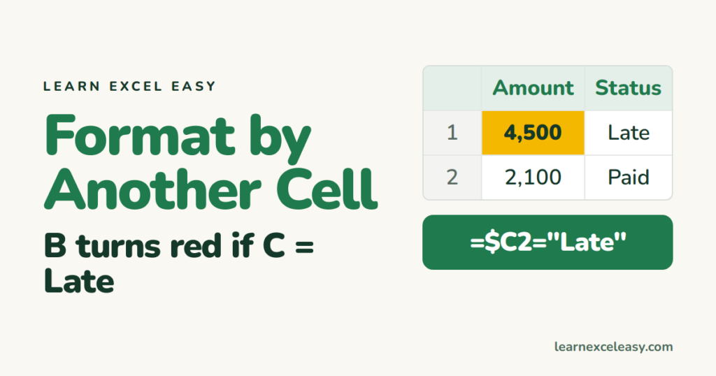
The built-in rules only look at the cell itself. To colour one cell based on another cell, use a formula rule.

Example: colour the amount when status is Late

1. Select the amounts, starting from the first data row: B2:B100.
2. Home › Conditional Formatting › New Rule › Use a formula to determine which cells to format.
3. Formula: =$C2="Late"
4. Format › Fill › red › OK › OK.

Why the $ is where it is

Write the formula as if for the first selected cell (B2). Excel moves it for every other cell like a copied formula.

• $C — always look at column C.
• 2 without $ — move down with each row.

More on $: absolute references.

Compare with a single target cell

Colour sales above the target typed in F1:

=B2>$F$1

Both $ signs — every cell compares with the same F1. Change F1 and the colours update.

Overdue dates

Colour the due date in C when it’s past and the invoice isn’t paid (D):

=AND($C2<TODAY(),$D2<>"Paid")

Colour the whole row

Select A2:F100 instead of one column, same formula with $C2. Full guide: highlight a row.

It colours the wrong cells

• You started the selection at row 1 but wrote the formula for row 2 — everything is off by one row.
• Missing $ before the column letter — the test drifts right.
• Check existing rules: Conditional Formatting › Manage Rules.

Basics: conditional formatting