
Convert a Table to a Normal Range in Excel (keep the formatting)
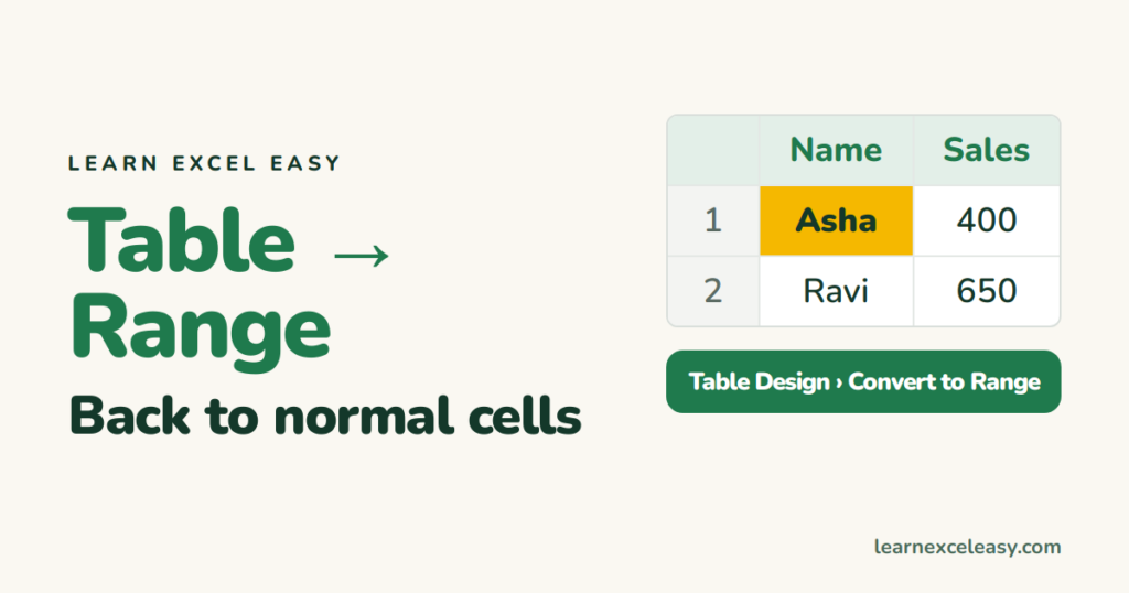
An Excel Table (Ctrl+T) adds filters, banded rows and auto-expanding formulas. Sometimes you want plain cells back — for example to merge cells or share with an old system.
Steps
- Click any cell inside the table.
- Table Design tab › Convert to Range.
- Click Yes.
Or right-click inside the table › Table › Convert to Range.
What stays and what goes
| Stays | Goes |
|---|---|
| All data | Filter arrows |
| Colours and banding (as normal formatting) | Automatic expansion for new rows |
| Formulas (converted to normal references) | The table name and structured references |
A formula like =SUM(Sales[Amount]) becomes =SUM(C2:C50) automatically.
Remove the colours too
Before converting: Table Design › Table Styles › click the drop-down › Clear (or pick “None” at the top). Then Convert to Range. Or after converting: select the cells › Home › Clear › Clear Formats (this also removes number formats).
Convert to Range is greyed out
- The sheet is protected — unprotect it first.
- The workbook is shared (legacy sharing) — tables can’t be converted while shared.
- You clicked outside the table.
Think twice
Tables make slicers, pivot tables and drop-down lists grow with your data. If the goal is just to remove the stripes, change the style to None and keep the table.

20 years with spreadsheets and enterprise systems. Writes one short, plain-English Excel lesson a day. Got an Excel question? learnexceleasycom@gmail.com
