Moving Average in Excel (formula and chart trendline)

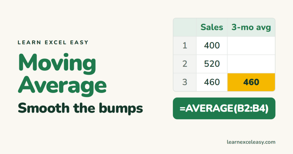
A moving (rolling) average smooths out ups and downs so the trend is easier to see.

3-month moving average

Sales in B2:B25. In C4 (the 3rd data row):

=AVERAGE(B2:B4)

Fill down. Each row averages itself and the two before — the range slides because it has no $ signs.

7-day or 12-month

Same idea with a bigger range: start in row 8 with =AVERAGE(B2:B8), or row 13 with =AVERAGE(B2:B13).

One formula from row 2

=IF(ROW()-ROW($B$2)+1<3,"",AVERAGE(OFFSET(B2,-2,0,3,1)))

Blank until there are 3 values. See OFFSET.

Period length in a cell

=AVERAGE(OFFSET(B2,1-$F$1,0,$F$1,1))

Change F1 from 3 to 6 and every row updates (start from row F1+1).

On a chart

1. Make a line chart of the sales.
2. Click the line › Chart Elements (+) › Trendline › More Options.
3. Choose Moving Average, set Period to 3.

Running average instead

Average of everything so far: =AVERAGE($B$2:B2). Related: running total.