How to Calculate a Z-Score in Excel

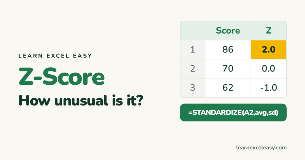
Z = (value − average) ÷ standard deviation. Z = 2 means two standard deviations above average; −1 means one below.

Step 1: average and standard deviation

E1: =AVERAGE(B2:B100)
E2: =STDEV.S(B2:B100)

Which STDEV? See standard deviation.

Step 2: the z-score

=STANDARDIZE(B2,$E$1,$E$2)

Or by hand: =(B2-$E$1)/$E$2. The $ signs keep the references fixed as you fill down — absolute references.

One formula, no helper cells

=(B2-AVERAGE(B$2:B$100))/STDEV.S(B$2:B$100)

Reading it

• Between −1 and 1: ordinary.
• Beyond ±2: unusual.
• Beyond ±3: likely an outlier — check it.

Flag outliers

=IF(ABS(C2)>3,"Check","")

Z-score to percentile

=NORM.S.DIST(C2,TRUE)

Format as %. Z = 1 → about 84%: higher than 84% of values (in bell-shaped data).

Colour them

Conditional Formatting › Color Scales on the Z column. Conditional formatting.