VLOOKUP Not Working? The 7 causes, in the order to check

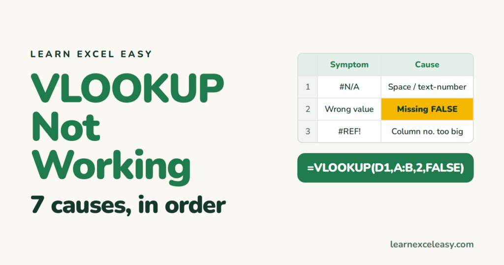
Check these in order. The first three fix 90% of cases.

1. Missing FALSE → wrong answers

=VLOOKUP(D1, A:B, 2) with no fourth part does an approximate match and returns nonsense from an unsorted list. Add , FALSE.

2. Extra spaces → #N/A

“Ana ” ≠ “Ana”. Test with =LEN(D1) vs =LEN(A5). Fix: =VLOOKUP(TRIM(D1), A:B, 2, FALSE) and TRIM the table too.

3. Number vs text → #N/A

Code 1001 as a number does not match “1001” as text. Signs: one is left-aligned. Fix: convert the column (text to number), or =VLOOKUP(TEXT(D1,"0"), A:B, 2, FALSE).

4. Lookup value not in the first column → #N/A

VLOOKUP only searches the leftmost column of the range you gave. If codes are in B and names in A, use INDEX MATCH or XLOOKUP.

5. Column number too big → #REF!

A:B has 2 columns; asking for column 3 gives #REF!. Widen the range or lower the number.

6. Range slid when copied down → #N/A on later rows

A1:B50 becomes A2:B51 on the next row. Lock it: $A$1:$B$50 (select it, press F4).

7. Formula shows as text

The cell is formatted as Text. Ctrl + 1 › General, then F2, Enter. See formula not calculating.

Still #N/A?

The value really is not there. Show it kindly: =IFERROR(VLOOKUP(...), "Not found").

Check it worked

Type a code you can see in the table. The right name appears. Type one that is not there — “Not found”.