How to Hide Columns in Excel (and unhide them later)

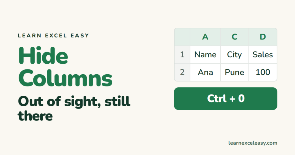
Hiding a column tucks it out of view. The data stays, formulas still use it, it just does not show or print.

Steps

1. Click the column letter, e.g. B. For several, click the first and Shift + click the last; for scattered ones hold Ctrl.
2. Right-click a selected letter › Hide. Or press Ctrl + 0.

The letters now jump A, C, D — B is hidden. A thin double line marks the spot.

Unhide

1. Select the columns either side: click A, Shift + click C.
2. Right-click › Unhide.

Everything hidden: click the corner triangle, then Ctrl + Shift + 0 or right-click any letter › Unhide.

Hide and show often? Use Group

1. Select the columns. Data › Group.
2. A − button appears above them. Click − to collapse, + to expand.

Better than hiding for helper columns you check now and then.

Check it worked

A formula that refers to the hidden column still shows its result. Printing skips the hidden column.

Common mistakes

Column A is hidden and you cannot select left of it. Type A1 in the Name Box (left of the formula bar), Enter, then Home › Format › Hide & Unhide › Unhide Columns.

Copy-paste includes hidden columns. To copy only what you see: select, F5 › Special › Visible cells only, then copy.