
IFERROR in Excel: hide #N/A and #DIV/0! errors
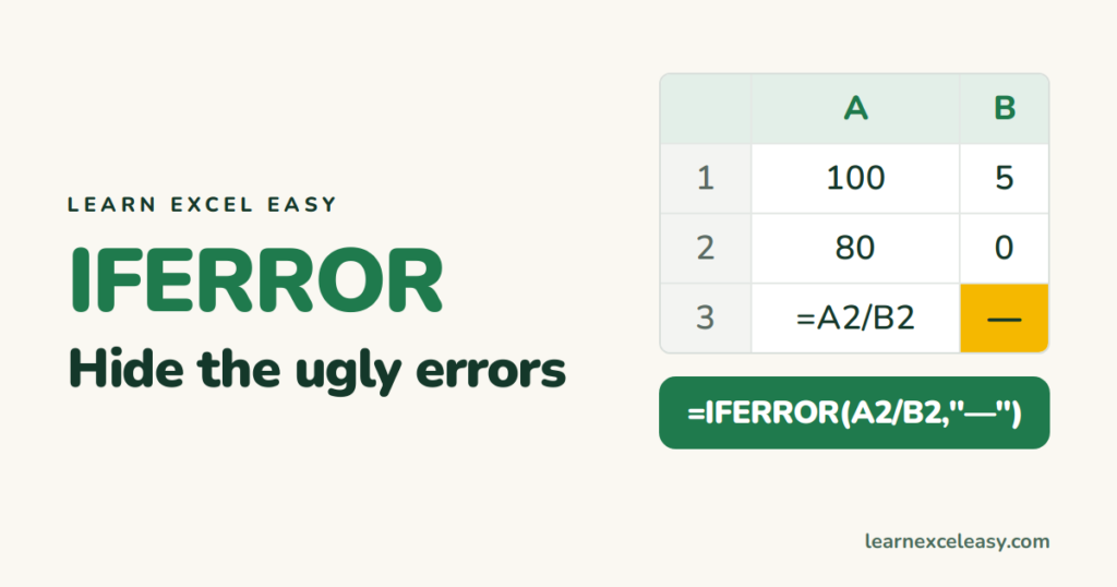
Errors like #N/A and #DIV/0! are correct but ugly. IFERROR lets you show something else — a dash, a zero, a message, or nothing.
The formula
=IFERROR(your_formula, what_to_show_instead)
Steps
- A formula that sometimes errors, e.g.
=A2/B2where B2 can be 0. - Wrap it:
=IFERROR(A2/B2, "—"). Enter.
Rows where B is 0 show a dash instead of #DIV/0!.
Lookups that find nothing
=IFERROR(VLOOKUP(D1, A:B, 2, FALSE), "Not found")
XLOOKUP has this built in as its 4th part, so it does not need IFERROR.
Show a blank
Use two quotes with nothing between: =IFERROR(A2/B2, "").
Show zero (careful)
=IFERROR(A2/B2, 0) lets SUM and AVERAGE keep working — but a zero looks like a real result. Prefer “” or a dash unless you need maths on it.
Check it worked
Type 0 into B2. The cell shows your replacement, not an error. Type 5 — the real answer comes back.
When NOT to use it
Wrapping everything hides typos too — a misspelled range name gives #NAME? and IFERROR silently blanks it. Use it on the final display formula, not while building.

20 years with spreadsheets and enterprise systems. Writes one short, plain-English Excel lesson a day. Got an Excel question? learnexceleasycom@gmail.com
